Interrupted Time Series for fixed-period interventions#
Interrupted time series experiments could be broken down into two types.
Interventions that occur at a point in time
Interventions that have a fixed period.
This notebook deals with the latter case, where there is no intervention up to a point where an intervention is in effect for a fixed period of time. Examples might include marketing promotions, price discounts, or public policy interventions.
When we are dealing with fixed-period interventions, we can make our interrupted time series experiment aware of this by providing treatment_end_time as a keyword argument. This then creates 3 distinct time periods:
Pre-intervention perior: Before any treatment has taken effect. This is what we fit our model to.
Intervention period: When treatment is active (from
treatment_timetotreatment_end_time)Post-intervention period: After treatment ends
This enables analysis of immediate effects, effect persistence, and decay patterns.
Note
For standard two-period ITS analysis (permanent interventions), see Bayesian Interrupted Time Series.
import matplotlib.pyplot as plt
import numpy as np
import pandas as pd

import causalpy as cp
%load_ext autoreload
%autoreload 2
%config InlineBackend.figure_format = 'retina'
seed = 42
Example: Marketing Campaign#
We simulate a 12-week marketing campaign with an immediate effect (+25 units) and partial persistence after it ends (+8 units, ~30% persistence).
Show code cell source
# Set up simulation parameters
rng = np.random.default_rng(seed)
n_weeks = 135  # 2 years of weekly data
dates = pd.date_range(start="2022-06-01", end="2024-12-31", freq="W")

# Baseline: trend + seasonality + noise
trend = np.linspace(100, 120, n_weeks)
season = 10 * np.sin(2 * np.pi * np.arange(n_weeks) / 52)  # Annual seasonality
noise = rng.normal(0, 5, n_weeks)
baseline = trend + season + noise

# Add intervention effect
treatment_idx = n_weeks // 2  # Start at midpoint
treatment_end_idx = treatment_idx + 12  # 12 weeks duration

y = baseline.copy()
y[treatment_idx:treatment_end_idx] += 25  # During intervention
y[treatment_end_idx:] += 8  # Post-intervention (persistence)

# Create DataFrame
df = pd.DataFrame(
    {
        "y": y,
        "t": np.arange(n_weeks),
        "month": dates.month,
    },
    index=dates,
)

treatment_time = dates[treatment_idx]
treatment_end_time = dates[treatment_end_idx]

print(f"Treatment starts: {treatment_time}")
print(f"Treatment ends: {treatment_end_time}")
print(f"Intervention period: {treatment_end_idx - treatment_idx} weeks")
print(f"Post-intervention period: {n_weeks - treatment_end_idx} weeks")
Treatment starts: 2023-09-17 00:00:00
Treatment ends: 2023-12-10 00:00:00
Intervention period: 12 weeks
Post-intervention period: 56 weeks
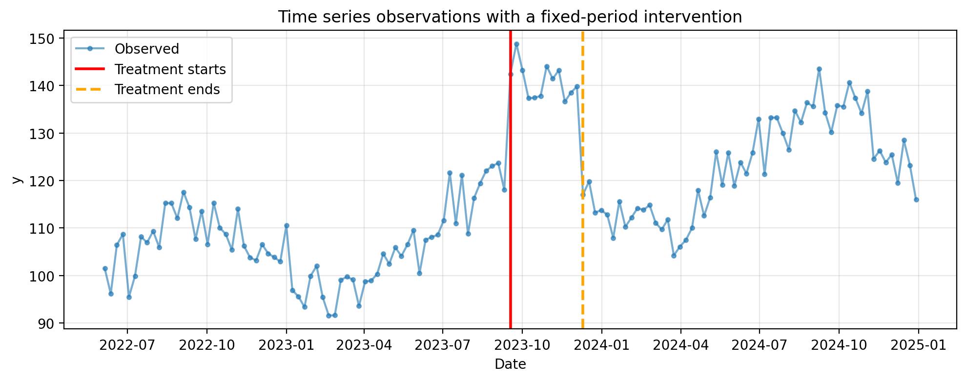
Let’s first visualize the raw time series data to get an intuitive sense of the intervention effect
Show code cell source
# Plot the raw data with treatment periods marked
fig, ax = plt.subplots(figsize=(10, 4))

ax.plot(df.index, df["y"], "o-", markersize=3, alpha=0.6, label="Observed")
ax.axvline(
    treatment_time, color="red", linestyle="-", linewidth=2, label="Treatment starts"
)
ax.axvline(
    treatment_end_time,
    color="orange",
    linestyle="--",
    linewidth=2,
    label="Treatment ends",
)

ax.set_xlabel("Date")
ax.set_ylabel("y")
ax.set_title("Time series observations with a fixed-period intervention")
ax.legend()
ax.grid(True, alpha=0.3)
plt.tight_layout()
plt.show()
Run the Analysis#
Specify treatment_end_time to enable three-period analysis:
result = cp.InterruptedTimeSeries(
    df,
    treatment_time=treatment_time,
    treatment_end_time=treatment_end_time,
    formula="y ~ 1 + t + C(month)",
    model=cp.pymc_models.LinearRegression(
        sample_kwargs={
            "random_seed": seed,
            "progressbar": False,
        }
    ),
)
Initializing NUTS using jitter+adapt_diag...
Multiprocess sampling (4 chains in 4 jobs)
NUTS: [beta, y_hat_sigma]
Sampling 4 chains for 1_000 tune and 1_000 draw iterations (4_000 + 4_000 draws total) took 2 seconds.
Sampling: [beta, y_hat, y_hat_sigma]
Sampling: [y_hat]
Sampling: [y_hat]
Sampling: [y_hat]
Sampling: [y_hat]
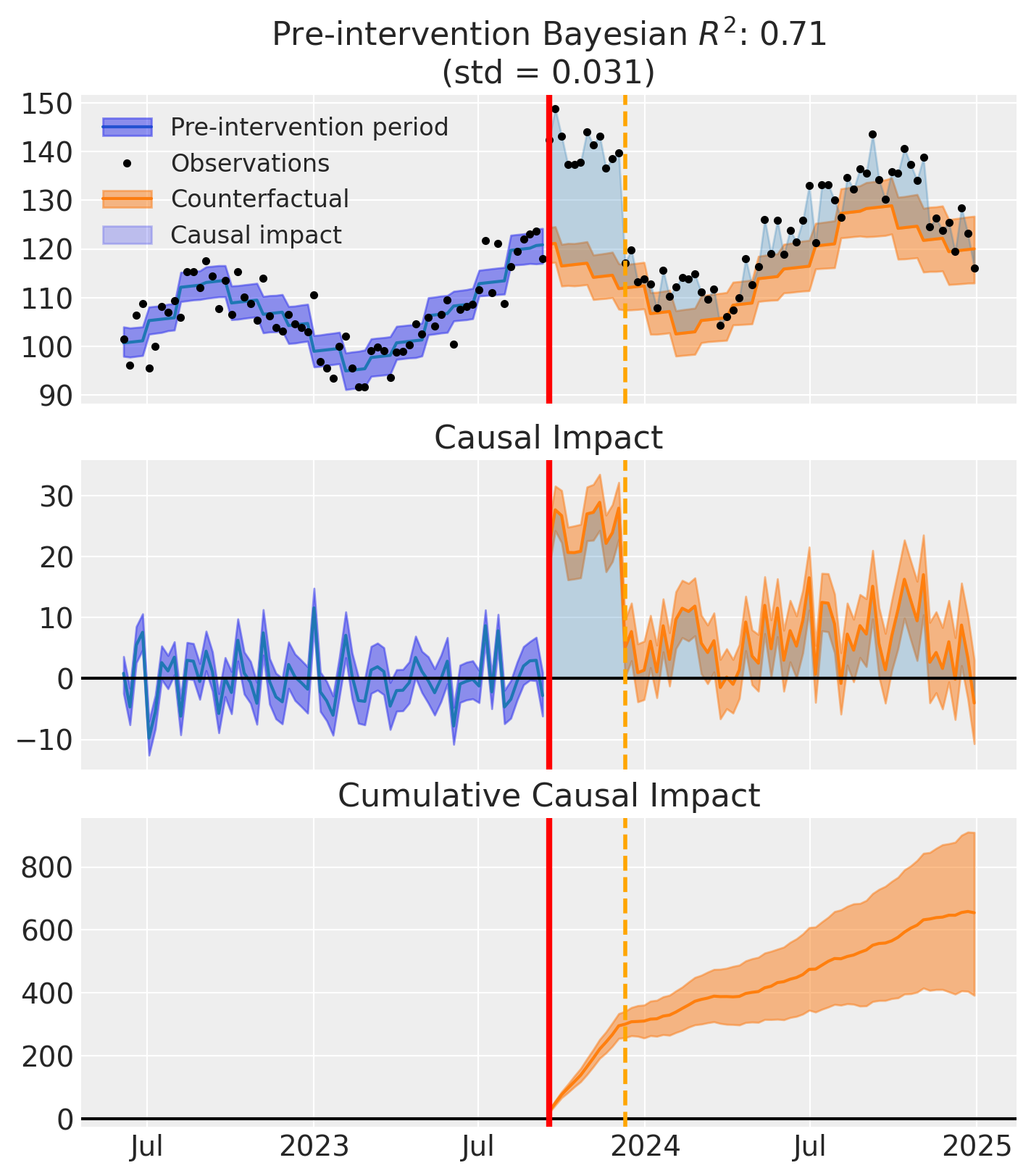
Visualization#
The three-period design visualization adds a vertical line to mark where the treatment ends:
Solid red line:
treatment_time(intervention start)Dashed orange line:
treatment_end_time(intervention end)
The plot shows three panels:
Top panel: Time series with observations, counterfactual predictions, and causal impact shading
Middle panel: Pointwise causal impact over time
Bottom panel: Cumulative causal impact
The vertical line at treatment_end_time clearly separates the intervention period from the post-intervention period, allowing you to visually assess effect persistence and decay.
fig, ax = result.plot()
plt.show()
Period-Specific Summaries#
Get separate summaries for each period using the period parameter:
# Intervention period
intervention_summary = result.effect_summary(period="intervention")
print(intervention_summary.text)
During the during intervention (2023-09-17 00:00:00 to 2023-12-03 00:00:00), the response variable had an average value of approx. 140.87. By contrast, in the absence of an intervention, we would have expected an average response of 116.28. The 95% interval of this counterfactual prediction is [112.90, 119.73]. Subtracting this prediction from the observed response yields an estimate of the causal effect the intervention had on the response variable. This effect is 24.59 with a 95% interval of [21.13, 27.97].

Summing up the individual data points during the during intervention, the response variable had an overall value of 1690.40. By contrast, had the intervention not taken place, we would have expected a sum of 1395.34. The 95% interval of this prediction is [1354.78, 1436.81].

The 95% HDI of the effect [21.13, 27.97] does not include zero. The posterior probability of a increase is 1.000. Relative to the counterfactual, the effect represents a 21.17% change (95% HDI [17.47%, 24.59%]).

This analysis assumes that the relationship between the time-based predictors and the response observed during the pre-intervention period remains stable throughout the post-intervention period. If the formula includes external covariates, it further assumes they were not themselves affected by the intervention. We recommend inspecting model fit, examining pre-intervention trends, and conducting sensitivity analyses (e.g., placebo tests) to support any causal conclusions drawn from this analysis.
# Post-intervention period
post_summary = result.effect_summary(period="post")
print(post_summary.text)
During the post-intervention (2023-12-10 00:00:00 to 2024-12-29 00:00:00), the response variable had an average value of approx. 122.63. By contrast, in the absence of an intervention, we would have expected an average response of 116.21. The 95% interval of this counterfactual prediction is [112.11, 120.44]. Subtracting this prediction from the observed response yields an estimate of the causal effect the intervention had on the response variable. This effect is 6.42 with a 95% interval of [2.19, 10.52].

Summing up the individual data points during the post-intervention, the response variable had an overall value of 6867.34. By contrast, had the intervention not taken place, we would have expected a sum of 6507.72. The 95% interval of this prediction is [6278.34, 6744.91].

The 95% HDI of the effect [2.19, 10.52] does not include zero. The posterior probability of a increase is 0.999. Relative to the counterfactual, the effect represents a 5.56% change (95% HDI [1.82%, 9.38%]).

This analysis assumes that the relationship between the time-based predictors and the response observed during the pre-intervention period remains stable throughout the post-intervention period. If the formula includes external covariates, it further assumes they were not themselves affected by the intervention. We recommend inspecting model fit, examining pre-intervention trends, and conducting sensitivity analyses (e.g., placebo tests) to support any causal conclusions drawn from this analysis.
Comparison Summary#
Use period='comparison' to get a comparative summary showing persistence metrics:
comparison_summary = result.effect_summary(period="comparison")
print(comparison_summary.text)
Effect persistence: The post-intervention effect (6.4, 95% HDI [2.2, 10.5]) was 26.1% of the intervention effect (24.6, 95% HDI [21.1, 28.0]), with a posterior probability of 1.00 that some effect persisted beyond the intervention period.
The comparison summary provides:
Post-intervention effect as percentage of intervention effect
Posterior probability that some effect persisted
HDI interval comparison between periods
Detailed Persistence Analysis#
The analyze_persistence() method automatically prints and returns a detailed summary of effect persistence:
persistence = result.analyze_persistence()
============================================================
Effect Persistence Analysis
============================================================

During intervention period:
  Mean effect: 24.59
  95% HDI: [21.13, 27.97]
  Total effect: 295.05

Post-intervention period:
  Mean effect: 6.42
  95% HDI: [2.19, 10.52]
  Total effect: 359.61

Persistence ratio: 0.261
  (26.1% of intervention effect persisted)
============================================================
# Access the returned dictionary:
print("\nAccessing results programmatically:")
print(f"  Mean effect during: {persistence['mean_effect_during']:.2f}")
print(f"  Mean effect post: {persistence['mean_effect_post']:.2f}")
print(
    f"  Persistence ratio: {persistence['persistence_ratio']:.3f} ({persistence['persistence_ratio'] * 100:.1f}%)"
)
print(f"  Total effect during: {persistence['total_effect_during']:.2f}")
print(f"  Total effect post: {persistence['total_effect_post']:.2f}")
Accessing results programmatically:
  Mean effect during: 24.59
  Mean effect post: 6.42
  Persistence ratio: 0.261 (26.1%)
  Total effect during: 295.05
  Total effect post: 359.61
Summary#
The three-period design enables analysis of temporary interventions:
Immediate effects:
effect_summary(period="intervention")analyzes effects during the active interventionPersistence:
effect_summary(period="post")measures how effects persist after the intervention endsComparison:
effect_summary(period="comparison")provides a comparative summary with persistence metricsDetailed analysis:
analyze_persistence()automatically prints and returns a detailed summary with mean effects, persistence ratio (as decimal), and total effects
The persistence ratio (e.g., 0.30 = 30%) indicates how much of the intervention effect “carried over” into the post-intervention period. Note that the ratio can exceed 1.0 if the post-intervention effect is larger than the intervention effect.
In practice, persistence effects could be caused by various mechanisms. For example, in marketing contexts, persistence might reflect brand awareness effects that continue to influence consumer behavior even after the promotional campaign ends.
We can get nicely formatted tables from our integration with the maketables package.
from maketables import ETable

ETable(result, coef_fmt="b:.3f")